What makes a YouTube video trend?
Contributors (in alphabetical order): Carla Lorente Anon, Yuqi He, Preethi Narayanan, Divya Umapathy, Shyam Krishnan Venkateswaran
Introduction/Background:
YouTube is an online video-sharing platform with billions of users, posting and watching content for entertainment and education. YouTube monetizes popular videos for the number of views as it increases the use and popularity of the platform itself. With our project, we hope to provide insights on how to make money on YouTube by analyzing trending video features and predicting the popularity of a video given certain features.
Motivation and methods
We want to help people monetize their content more effectively on YouTube by increasing their popularity on the platform! To that end, we carry out the following analyses:
-
PCA: to reduce dimension of features through capturing variation and visualize correlation between different features
-
DBSCAN: to find the popular time published and optimal length, number of capital letters, and punctuation in video title
-
Linear Regression: predict the views based upon any other correlated features
-
Multiple Regression: to predict the popularity of a video solely based on the title's characteristics (length, capital letters, and puctuation)
-
Gradient Boosting Regressor: To build an ensemble regressor to predict the number of views and rank feature importances
Dataset:
-> https://www.kaggle.com/datasnaek/youtube-new
This dataset includes several months of data on daily trending YouTube videos. Data includes the video title, channel title, publish time, tags, views, likes and dislikes, description, and comment count for up to 200 trending videos per day for several regions. More information like the channel’s age, channel's video count, and subscriber count have been added using the YouTube API. From this dataset, we will only be using the USA's, Canada's, and Great Britain's trending video data.
YouTube API
We also augment the available data with our own data scavenged from YouTube using its APIs. We wrote a script to fetch the top 200 trending videos from USA, Canada and Great Britain everyday for roughly a month. In addition, the channel information was also fetched and compiled with the data from Kaggle.
Cleaning up the data
- Languages: Youtube fosters content from all around the world in numerous languages. We discarded video entries in the dataset that do not have English titles to facilitate the analysis of the data. (see code)
- Handling duplicates: Several videos are in trending charts for multiple days. Therefore, we retained only one copy of each video, the version with the highest number of views.
- Null entries: videos with ratings disabled and comments disabled were removed.
- Handling dates and time: We parsed the dates and times in YouTube's native format to formats suitable for machine learning algorithms (floats and integets) (see code)
- Handling outliers: To gain insights for the majority of the data, any data points that were outside +/-2 standard deviations from the mean were eliminated.
Data Format
The csv format of final file that contains both Old and New data:
| 1. regionTrending | 12. videoDislikes | 23. thumbnail_link |
| 2. trendingRank | 13. videoCommentCount | 24. comments_disabled |
| 3. timeFetched | 14. videoDescription | 25. ratings_disabled |
| 4. videoId | 15. videoLicenced | 26. video_error_or_removed |
| 5. videoTitle | 16. channelTitle | 27. publishDateCorrectFormat |
| 6. videoCategoryId | 17. channelId | 28. trendingDateCorrectFormat |
| 7. videoPublishTime | 18. channelDescription | 29. dayDifference |
| 8. videoDuration | 19. channelPublishedAt | 30. publishedZTime |
| 9. videoTags | 20. channelViewCount | 31. publishedZTimeFloat |
| 10. videoViews | 21. channelSubsCount | 32. publishedDayOfWeek |
| 11. videoLikes | 22. channelVideoCount | 33. newOrOldData |
Data Analysis
Correlation
First, an analysis of the correlation between different variables was performed. Looking at the first row, it is seen that only likes, dislikes and comment count are correlated with the number of views of a video.

Figure 1: Correlation Table
Statistical Summary
This analysis is useful to potentially identify any outliers in the data.

Figure 2: Statistical Summary
Category ID Analysis
The category ID represents the content of the video (Click here to see the different categories).
- Categories with high number of views: "Film & Animation", "Music", "News and Politics", and "Entertainment"
- Categories with least number of views: "Nonprofits & Activism" and "Shorts"
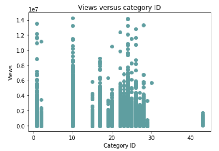
Figure 3: Views versus Category ID
Principal Component Analysis(PCA)
We selected some properties from the original video dataset as features of videos, including trending rank, video category, number of views, likes, and dislikes, number of comments, publish time, and video channel related features. For features like the duration of video and the publish time, we preprocessed our data such that they are represented in the same unit (seconds) and in a 24-hour time scale.
We combined all 12 features into a training dataset and apply PCA. PCA was used to reduce the dimension of features through capturing variation. Here is the cumulative explained variance plot.
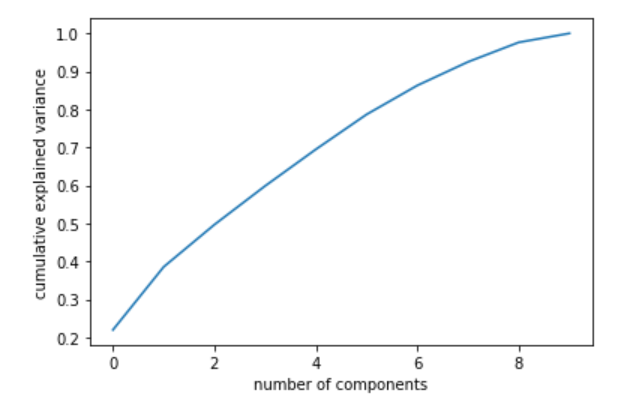
Figure 4: PCA variance plot
From the plot, we can see that at 6 components, we will get a desired cumulative explained variance(0.9). We also made two component PCA scatter plots to give us some visualizations.
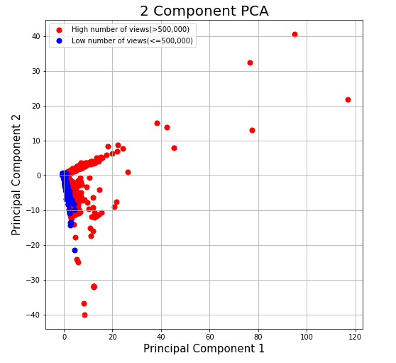
Figure 5: PCA number of views plot
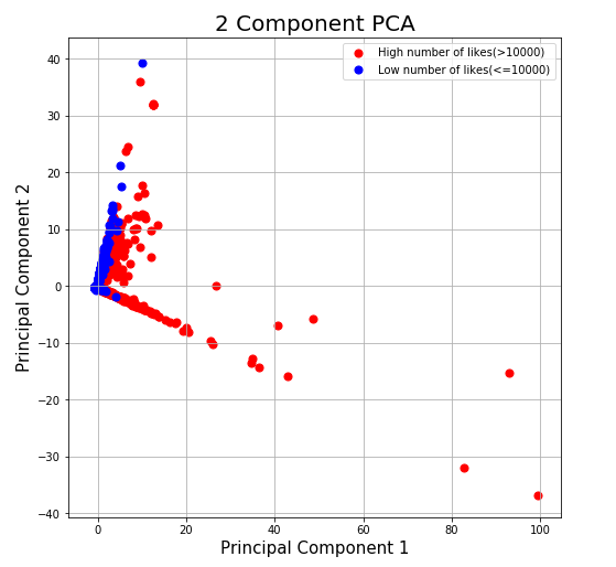
Figure 6: PCA number of likes plot
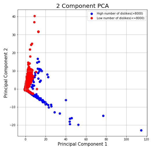
Figure 7: PCA number of dislikes plot
From the scatter plots, we can see that the number of views, likes, and dislikes are correlated. Low number of views, low number of likes, and low number of dislikes are all clustered at the middle-left part of the graph.
DBSCAN
Publishing Times
Using DBSCAN clustering on the video views and publishing time features, we can see that the optimal time frame to publish videos on YouTube is from about 1:00 pm to 7:00 pm GMT with the peak time between 5:00 pm - 7:00 pm; however, we did find many noise points and the clusters found were quite low in view count. (see code)
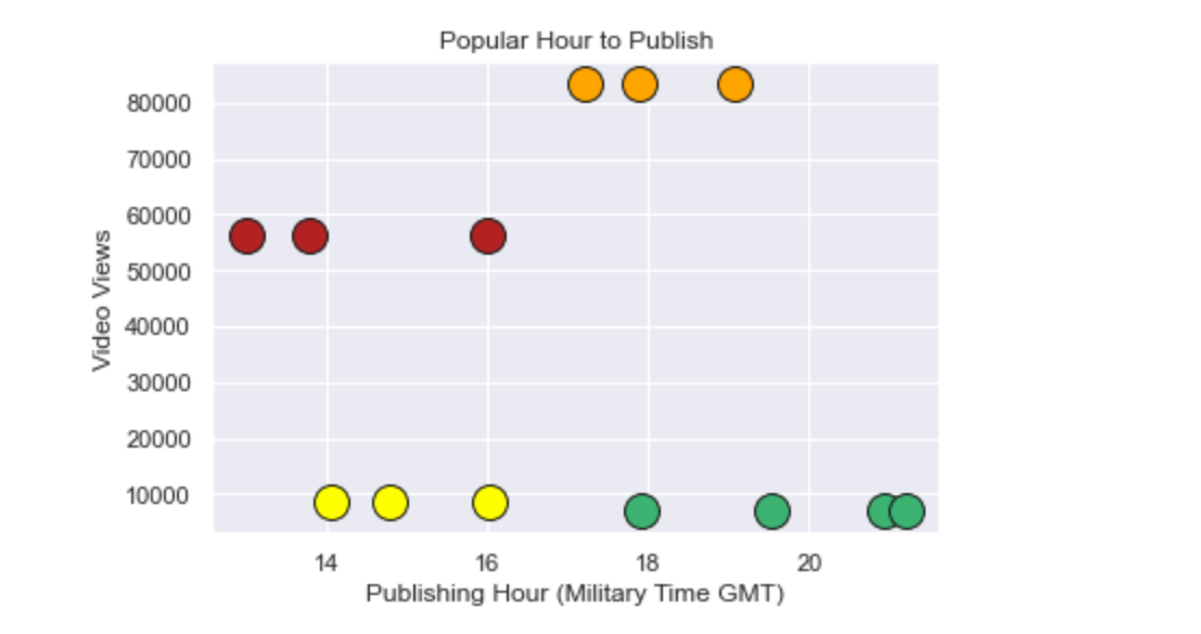
Figure 8.1: DBSCAN Hour Published
Video Titles
After using DBSCAN clustering on three different characteristics of a video title (length, number of capital letters,and number of exclamation/question marks) we can see that the results in the graphs below are different than we originally expected. (see code)
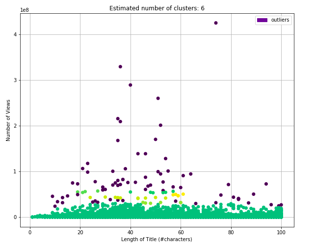
Figure 8.2: DBSCAN Title Length
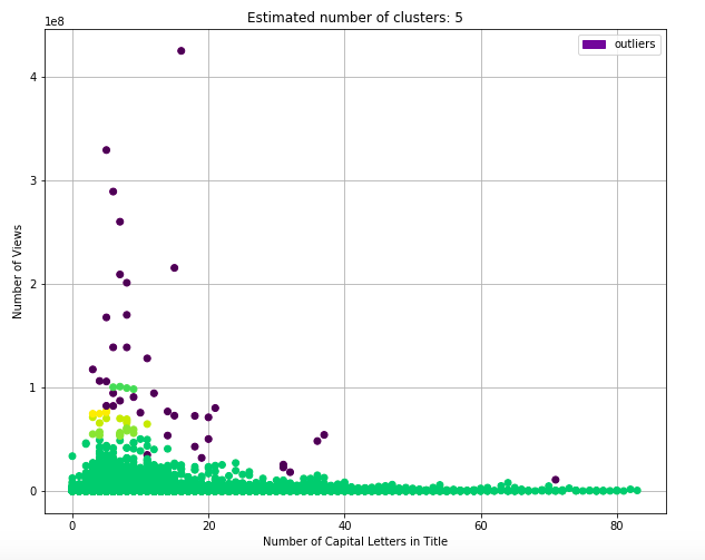
Figure 8.3: DBSCAN Capital Letters
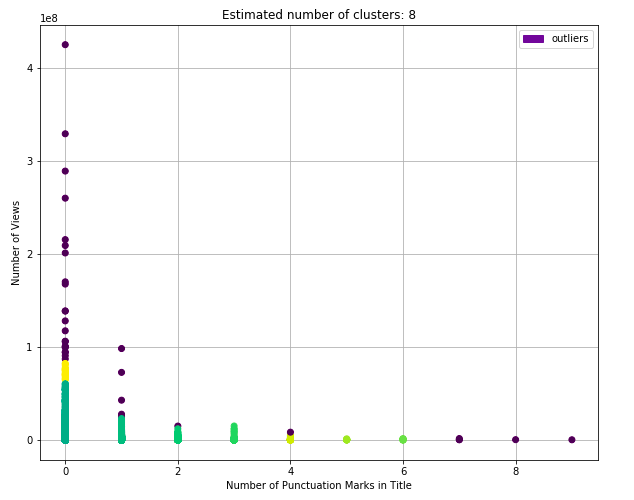
Figure 8.4: DBSCAN Punctuation Marks
The clusters for majority of the graphs are evenly distributed along the x axis, showing very little correlation to the number of views. But, there are a couple clusters higher up on the graph that show that titles with lengths around 40 characters, minimal capital letters, and minimal punctuation marks are the videos accumulating more views. As a conclusion, there is little relation seen between the factors, but there is some evidence pointing to certain title formats.
Linear Regression
Histograms
A basic histogram of the number of views, likes and dislikes was plotted. As it is appreciated on the graphs below, the three graphs are heavily skewed which is understandable — most common YouTubers probably won’t have that many views, likes and dislikes. Ideally, the data should resemble a Gaussian distribution. Luckily, a log tranformation can be applied to the number of views, likes and dislikes to achieve that.
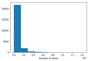
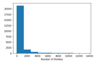
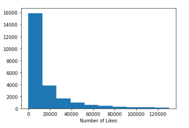
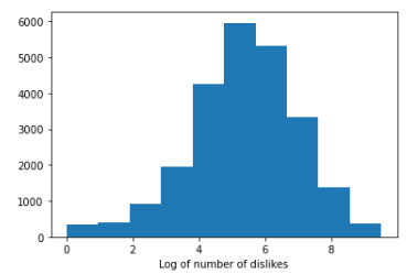
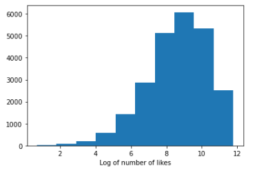
Linear Regression
Using this 3 histograms above, a linear regression of the log number of views versus the log number of likes and dislikes can be plotted (see code). As expected, both correlations show an R^2 greater than 0.6, showing a big correlation between both the number of likes and dislikes and the number of views of a video.
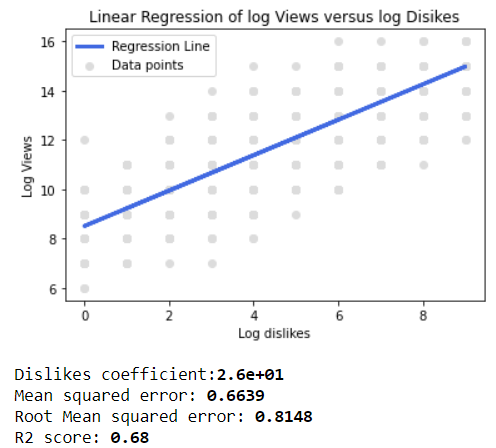
Figure 9: Linear regression of log views versus log dislikes
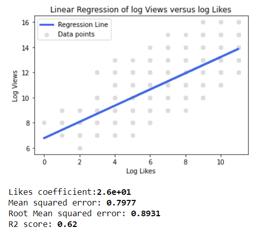
Figure 10: Linear regression of log views versus log likes
This analysis was only performed on these 2 variables since no other variables appear to correlate with the number of views of a video. For example, when performing the linear regression of views versus the title length, an R^2 close to 0 is obtained.
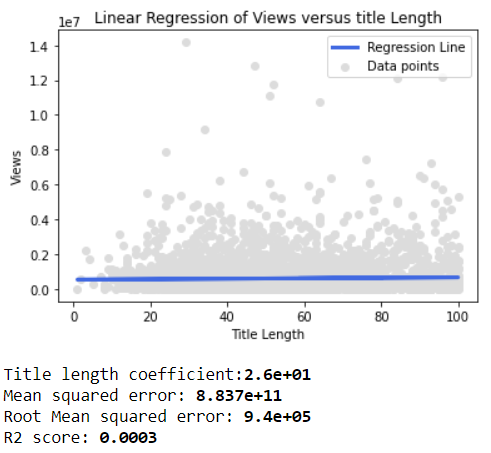
Figure 11: Linear regression of views versus title length
Multiple Regression
Data Modifications
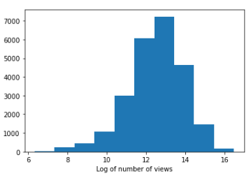
Data regarding number of views was originally very skewed, so we removed any outliers and took the log of the number of views. This resulted in a Gaussian distribution for the number of views, which is ideal for any modeling. The below graphs show the data distribution before and after applying the log function.
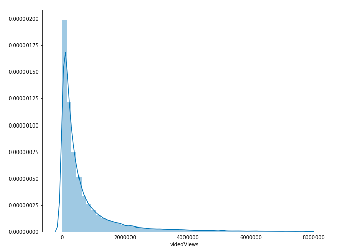
Figure 12: Multiple Regression Skewed Data
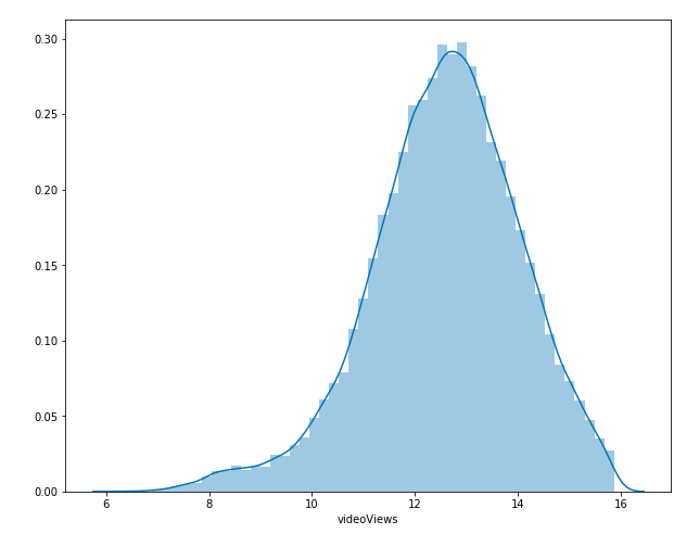
Figure 13: Multiple Regression Modified Data
Multiple Regression Analysis
We used three parameters versus the number of views on a video (title length, number of capital letters, number of punctuations marks). This would have resulted in a 3-dimensional regression model in a 4-dimensional space. As it is difficult to understand a 4-dimensional model, the following graphs show the regression models of just two parameters each versus the log of the number of views. (see code)
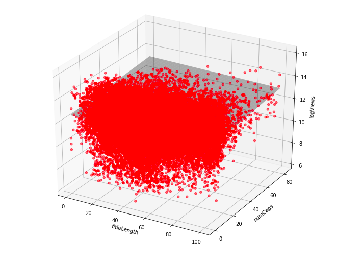
Figure 14: Multiple Regression Length vs Number of Capital Letters
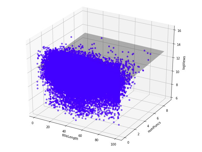
Figure 15: Multiple Regression Length vs Number of Punctuation Marks
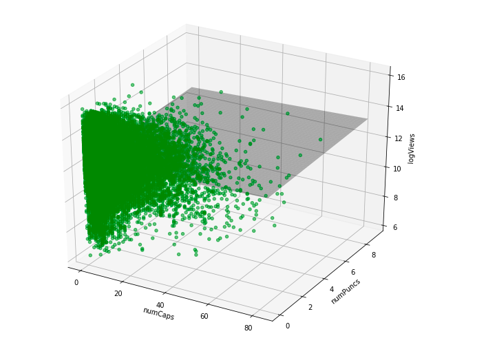
Figure 16: Multiple Number of Capital Letters vs Number of Punctuation Marks
As can be seen above, the grey plane in each of the graphs is the regression model that fits the set of data points the best. Since our data points are fairly spread out and do not show much correlation to the number of views, the fitted planes are relatively flat, and center around the area where most of the data points are in order to at least fit for a majority of videos.
Result Analysis
As a representation of the accuracy of our model, the below graph shows a comparison of the actual number views versus the predicted number of views for a random set of data points.
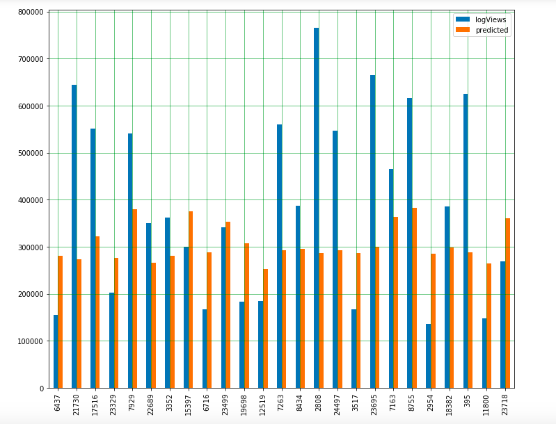
Figure 17: Predicted Views vs Actual Views
In the below graph, where it shows the error in prediction based on the number of actual views, it can be seen that the lower the actual number of views a video has, the more accurate this model will be in its predictions.
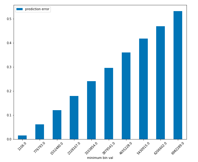
Figure 18: Multiple Regression Model Accuracy
In conclusion, we see that the characteristics of a video title actually have a much smaller effect on the popularity of a video than we originally believed and has an incredibly low correlation with the number of views, especially on videos with extremely high view count.
Gradient Boosting Regressor
Gradient Boosting Regressor is a form of tree ensemble model which builds an ensemble of weak prediction models. A new tree is trained at each step additively over the previous stage with the loss function as the residual error from previous stage.
Model used: The sklearn.ensemble.GradientBoostingRegressor model from sklearn module is used. The module also provides a method to visualize the importance of individual features after the model is trained. We use this to infer the most important contributors in predicting the number of views of a video (See here).
Data Preparation: The data collected using the YouTube API is used to train and test the model with the logarithm of number of views of a video as the target label. Only the videos that have a view count between 1000 and 10 million are used. Sample of the data used is shown:
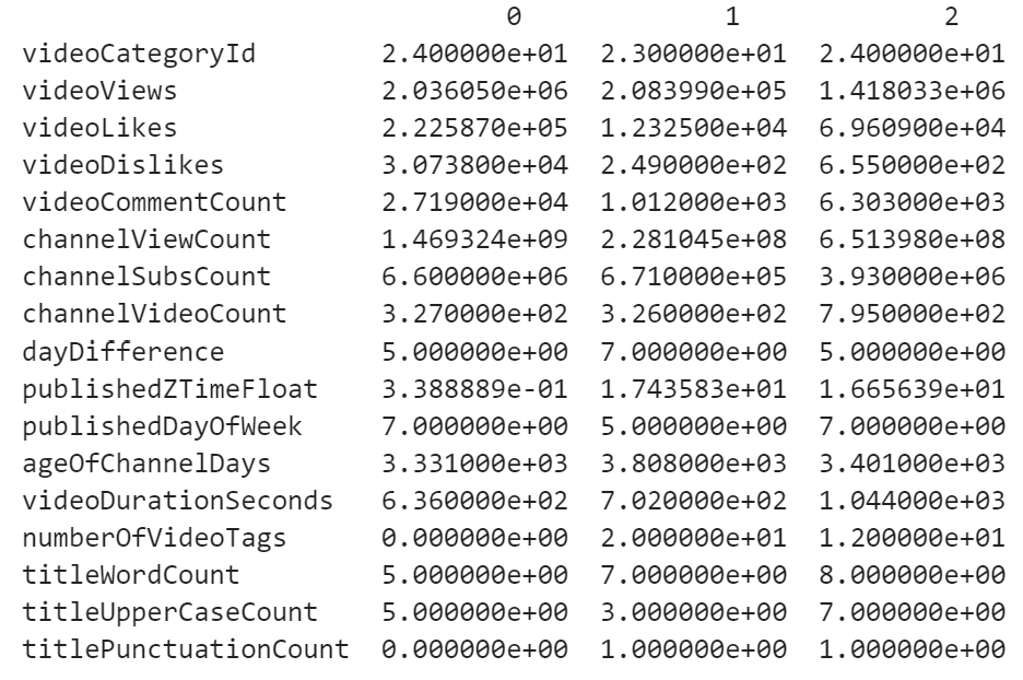
Figure 19: Sample of data for analysis
Model performance and Feature importance
With all the above listed features, the model has an RMSE of 772445 views. We infer from the plot that the number of likes and dislikes are the most important features in predicting the number of views.
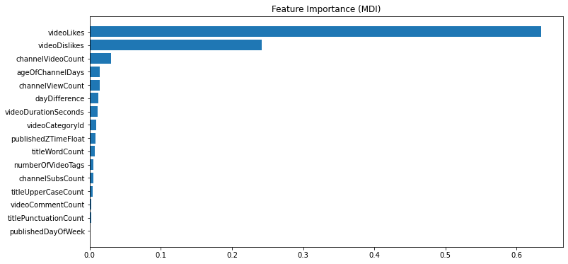
Figure 20: Feature importance-1
While this is intuitive, this does not serve as a good model for prediction since likes, dislikes, age of video and comments are not known in advance. After removing these features, the feature importance is plotted below:
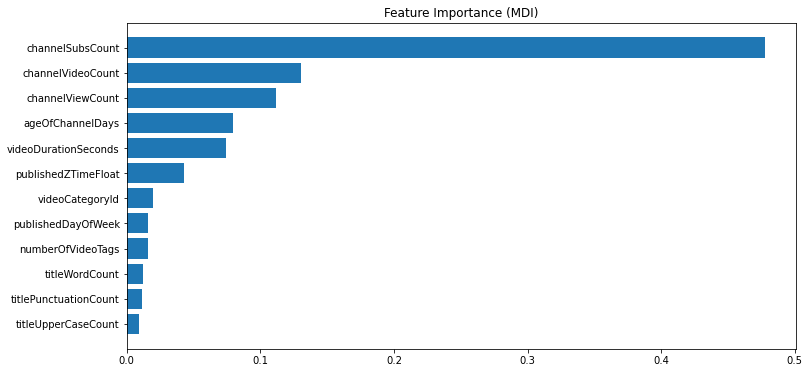
Figure 21: Feature importance-2
It is seen that the channel subscriber count, the number of videos, total views on the channel, and age of the channel are the most important predictors.
Conclusion
From the analyses we carried out, following are the key insights and results:
- Categories with high number of views: Film & Animation, Music, Entertainment and News and Politics.
- Categories with least number of views: Nonprofits & Activism and Shorts
- 1:00 pm to 7:00 pm GMT is a popular time frame to publish videos so they trend, especially between 5:00 pm-7:00 pm. There is no optimal title length. Fewer (or none) capital letters and punctuation in video title is optimal.
- There is a relationship between number of dislikes, number of likes, and number of views.
- The video title plays a minor role in the popularity of the most popular videos. But, for the less exposed or advertised videos, keeping to minimal capital letters and punctuation can help boost views slightly.
- The channel's popularity plays a major role in determining the popularity of a video. Particularly, the channel subscriber and view count, age of channel and channel video count are dominant factors.
Future Work
The following are a few possible directions in which our work can be extended:
- Analysis of the impact of keywords in the title on number of views
- Deeper analysis of relation between channel popularity and video popularity
- Estimating potential size of audience for a given video type (Music, Movie trailer, etc), language among other features.
Individual Contributions
Carla: Data Analysis, Cleaning data and Linear Regression
Yuqi: Principal Component Analysis
Preethi: DBSCAN and Multiple Regressor
Divya: Finding dataset, Cleaning data and DBSCAN
Shyam: Cleaning/Augmenting data using API and Gradient Boosting Regressor
References:
[1] Gill, Phillipa et al. "Youtube traffic characterization: a view from the edge." Proceedings of the 7th ACM SIGCOMM conference on Internet measurement. 2007.
[2] F Figueiredoet al "The tube over time: characterizing popularity growth of youtube videos." Proceedings of the fourth ACM international conference on Web search and data mining. 2011.
[3] G. Chatzopoulou et al, "A First Step Towards Understanding Popularity in YouTube," INFOCOM IEEE Conference on Computer Communications Workshops, CA, 2010
[4] Coding, Sigma. “How to Build a Linear Regression Model in Python | Part 1.” Youtube, Apr. 2019, www.youtube.com/watch?v=MRm5sBfdBBQ.
[5] "DBSCAN Clustering Easily Explained with Implementation." Youtube, https://www.youtube.com/watch?v=C3r7tGRe2eI&t=942s
[6] "Multiple Regression Analysis in Python | Part 1." Youtube Apr 27, 2019 https://www.youtube.com/watch?v=M32ghIt1c88
[7] "Youtube Views Predictor." Aravind Srinivasan, December 12, 2017 https://towardsdatascience.com/youtube-views-predictor-9ec573090acb
